Difference between Normalization and Partitioning in DBMS/SQL

Partitioning

Partitioning a database improves performance and simplifies maintenance. By splitting a large table into smaller, individual tables, queries that access only a fraction of the data can run faster because there is less data to scan. Maintenance tasks, such as rebuilding indexes or backing up a table, can run more quickly.

Partitioning can be achieved without splitting tables by physically putting tables on individual disk drives. Putting a table on one physical drive and related tables on a separate drive can improve query performance because, when queries that involve joins between the tables are run, multiple disk heads read data at the same time. SQL Server filegroups can be used to specify on which disks to put the tables.

Normalization 

Database Normalization is a technique of organizing the data in the database. Normalization is a systematic approach of decomposing tables to eliminate data redundancy(repetition) and undesirable characteristics like Insertion, Update and Deletion Anomalies. It is a multi-step process that puts data into tabular form, removing duplicated data from the relation tables.

Normalization is used for mainly two purposes,
Eliminating redundant(useless) data.
Ensuring data dependencies make sense i.e data is logically stored.

Database normalization involves designing the tables in the database to reduce or eliminate duplicated data. Normalization is a logical database design issue.

Horizontal partitioning is the process of breaking a large monolithic table into a series of smaller subtables which can be queried faster and managed more effectively by the DBMS. (This is what most people mean when they talk about "partitioning").

Vertical partitioning is the process of using multiple tables to store the data for a single entity; thus, instead of a single table with 100 columns you might have 4 tables with 25 columns each. Reasons for vertical partitioning might include storing large columns (e.g. BLOBs) or infrequently used columns on inexpensive-but-slow storage devices, while storing more-frequently-accessed columns on faster-but-more-expensive storage devices.

Partitioning is a physical database design issue.

• Why is a database normalized?
• What are the types of normalization?
• Why is database normalization important?
• What is database denormalization?
• Why would we denormalize a database?

So, let’s get started with normalization concepts…

According to Wikipedia …

“Database normalization is the process of restructuring a relational database in accordance with a series of so-called normal forms in order to reduce data redundancy and improve data integrity. It was first proposed by Edgar F. Codd as an integral part of his relational model.

Normalization entails organizing the columns (attributes) and tables (relations) of a database to ensure that their dependencies are properly enforced by database integrity constraints. It is accomplished by applying some formal rules either by a process of synthesis (creating a new database design) or decomposition (improving an existing database design).”

Database normalization

Database Normalization is a process and it should be carried out for every database you design. The process of taking a database design, and apply a set of formal criteria and rules, is called Normal Forms.

The database normalization process is further categorized into the following types:

1. First Normal Form (1 NF)
2. Second Normal Form (2 NF)
3. Third Normal Form (3 NF)
4. Boyce Codd Normal Form or Fourth Normal Form ( BCNF or 4 NF)
5. Fifth Normal Form (5 NF)
6. Sixth Normal Form (6 NF)

One of the driving forces behind database normalization is to streamline data by reducing redundant data. Redundancy of data means there are multiple copies of the same information spread over multiple locations in the same database. 

The drawbacks of data redundancy include:

1. Data maintenance becomes tedious – data deletion and data updates become problematic
2. It creates data inconsistencies
3. Insert, Update and Delete anomalies become frequent. An update anomaly, for example, means that the versions of the same record, duplicated in different places in the database, will all need to be updated to keep the record consistent
4. Redundant data inflates the size of a database and takes up an inordinate amount of space on disk

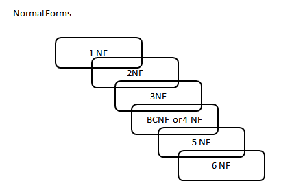
Normal Forms

This article is an effort to provide fundamental details of database normalization. The concept of normalization is a vast subject and the scope of this article is to provide enough information to be able to understand the first three forms of database normalization.

1. First Normal Form (1 NF)
2. Second Normal Form (2 NF)
3. Third Normal Form (3 NF)

A database is considered third normal form if it meets the requirements of the first 3 normal forms.

First Normal Form (1NF):

The first normal form requires that a table satisfies the following conditions:

1. Rows are not ordered
2. Columns are not ordered
3. There is duplicated data
4. Row-and-column intersections always have a unique value
5. All columns are “regular” with no hidden values

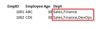
In the following example, the first table clearly violates the 1 NF. It contains more than one value for the Dept column. So, what we might do then is go back to the original way and instead start adding new columns, so, Dept1, Dept2, and so on. This is what’s called a repeating group, and there should be no repeating groups. In order to bring this First Normal Form, split the table into the two tables. Let’s take the department data out of the table and put it in the dept table. This has the one-to-many relationship to the employee table.

Let’s take a look at the employee table:

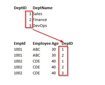
Now, after normalization, the normalized tables Dept and Employee looks like below:

Second Normal Form and Third Normal Form are all about the relationship between the columns that are the keys and the other columns that aren’t the key columns.

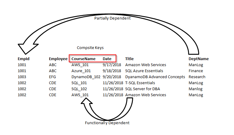
Second Normal Form (2NF):

An entity is in a second normal form if all of its attributes depend on the whole primary key. So this means that the values in the different columns have a dependency on the other columns.

1. The table must be already in 1 NF and all non-key columns of the tables must depend on the PRIMARY KEY
2. The partial dependencies are removed and placed in a separate table

Note: Second Normal Form (2 NF) is only ever a problem when we’re using a composite primary key. That is, a primary key made of two or more columns.

The following example, the relationship is established between the Employee and Department tables.

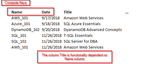
In this example, the Title column is functionally dependent on Name and Date columns. These two keys form a composite key. In this case, it only depends on Name and partially dependent on the Date column. Let’s remove the course details and form a separate table. Now, the course details are based on the entire key. We are not going to use a composite key.

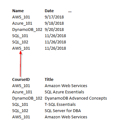
Third Normal Form (3NF):

The third normal form states that you should eliminate fields in a table that do not depend on the key.

1. A Table is already in 2 NF
2. Non-Primary key columns shouldn’t depend on the other non-Primary key columns
3. There is no transitive functional dependency

Consider the following example, in the table employee; empID determines the department ID of an employee, department ID determines the department name. Therefore, the department name column indirectly dependent on the empID column. So, it satisfies the transitive dependency. So this cannot be in third normal form.

In order to bring the table to 3 NF, we split the employee table into two.

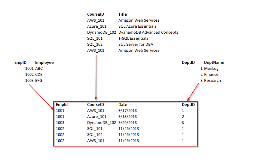
Now, we can see the all non-key columns are fully functionally dependent on the Primary key.

Although a fourth and fifth form does exist, most databases do not aspire to use those levels because they take extra work and they don’t truly impact the database functionality and improve performance.

Denormalization

According to Wikipedia…

“Denormalization is a strategy used on a previously-normalized database to increase performance. In computing, denormalization is the process of trying to improve the read performance of a database, at the expense of losing some write performance, by adding redundant copies of data or by grouping data.[1][2] It is often motivated by performance or scalability in relational database software needing to carry out very large numbers of read operations. Denormalization should not be confused with Unnormalized form. Databases/tables must first be normalized to efficiently denormalize them.”

Database normalization is always a starting point for denormalization. Denormalization is a type of reverse engineering process that can apply to retrieve the data in the shortest time possible.

Let us consider an example; we’ve got an Employee table that in-house an email and a phone number columns. Well, what happens if we add another email address column, another phone number? We tend to break First Normal Form. It’s a repeating group. But in general, it is easy to have those columns created (Email_1, and Email_2 column), or having (home_phone and mobile_phone) columns, rather than having everything into multiple tables and having to follow relationships. The entire process is referred to as a denormalization.

Summary

Thus far, we’ve discussed details of the Relational Database Management System (RDBMS) concepts such as Database Normalization (1NF, 2NF, and 3NF), and Database Denormalization

Again, the basic understandings of database normalization always help you to know the relational concepts, a need for multiple tables in the database design structures and how to query multiple tables in a relational world. It is a lot more common in data warehousing type of scenarios, where you’ll probably work on a process to de-normalize the data. Denormalized data is actually much more efficient to query than normalized data. 

Taking the database design through these three steps will vastly improve the quality of the data.

SQL PARTITION BY

Summary: in this tutorial, you will learn how to use the SQL PARTITION BY clause to change how the window function calculates the result.

SQL PARTITION BY clause overview

The PARTITION BY clause is a subclause of the OVER clause. The PARTITION BY clause divides a query’s result set into partitions. The window function is operated on each partition separately and recalculate for each partition.

The following shows the syntax of the PARTITION BY clause:

window_function ( expression ) OVER (

    PARTITION BY expression1, expression2, ...

    order_clause

    frame_clause

)

You can specify one or more columns or expressions to partition the result set. The expression1, expression1, etc., can only refer to the columns derived by the FROM clause. They cannot refer to expressions or aliases in the select list.

The expressions of the PARTITION BY clause can be column expressions, scalar subquery, or scalar function. Note that a scalar subquery and scalar function always returns a single value.

If you omit the PARTITION BY clause, the whole result set is treated as a single partition.

PARTITION BY vs. GROUP BY

The GROUP BY clause is used often used in conjunction with an aggregate function such as SUM() and AVG(). The GROUP BY clause reduces the number of rows returned by rolling them up and calculating the sums or averages for each group.

For example, the following statement returns the average salary of employees by departments:

1 2 3 4 5 6 7 8 9

SELECT     department_id,     ROUND(AVG(salary)) avg_department_salary FROM     employees GROUP BY     department_id ORDER BY     department_id;

The following picture shows the result:

The PARTITION BY clause divides the result set into partitions and changes how the window function is calculated. The PARTITION BY clause does not reduce the number of rows returned.

The following statement returns the employee’s salary and also the average salary of the employee’s department:

1 2 3 4 5 6 7 8 9

SELECT     first_name,     last_name,     department_id,     ROUND(AVG(salary) OVER (         PARTITION BY department_id     )) avg_department_salary FROM     employees;

Here is the partial output:

In simple words, the GROUP BY clause is aggregate while the PARTITION BY clause is analytic.

What is a Self Join? Explain with Example

Answer: A self-join is simply a normal SQL join that joins one table to itself. Joining a table to itself can be useful when you want to compare values in a column to other values in the same column.

Question: Is Self Join Inner Join or Outer Join?

Answer: A self-join can be an inner join or an outer join or even a cross join. A table is joined to itself based upon a column that have duplicate data in different rows.

Question: What is a practical use of the Self Join in the real world?

Answer: The best example of self join in the real world is when we have a table with Employee data and each row contains information about employee and his/her manager. You can use self join in this scenario and retrieve relevant information. Let us see an example, over here.

Let us first create the same table for an employee.

One of the columns in the same table contains the ID of the manger, who is also an employee for the same company. Now all the employees and their managers are present in the same table. Let us see how Self Join works in the real world scenario now.

1 2 3 4 5 6 7 8 9 10 11 12 13 14 15 16 17 18 19 20 21 22 23 24 25 26 27

USE TempDb GO -- Create a Table CREATE TABLE Employee( EmployeeID INT PRIMARY KEY, Name NVARCHAR(50), ManagerID INT ) GO -- Insert Sample Data INSERT INTO Employee SELECT 1, 'Mike', 3 UNION ALL SELECT 2, 'David', 3 UNION ALL SELECT 3, 'Roger', NULL UNION ALL SELECT 4, 'Marry',2 UNION ALL SELECT 5, 'Joseph',2 UNION ALL SELECT 7, 'Ben',2 GO -- Check the data SELECT * FROM Employee GO

Let us now connect the Employee table with itself with the help of INNER JOIN.

1 2 3 4 5 6

-- Inner Join SELECT e1.Name EmployeeName, e2.name AS ManagerName FROM Employee e1 INNER JOIN Employee e2 ON e1.ManagerID = e2.EmployeeID GO

In the result set, we can see that all the employees who have a manager are visible. Though the above solution has one limitation. The limitation is that we are not able to find out the top manager of the company in our result set. Inner join does not display any result which does not have a manager id in our scenario.

Next let us convert Inner Join to Outer Join and then see the result set.

1 2 3 4 5 6

-- Outer Join SELECT e1.Name EmployeeName, ISNULL(e2.name, 'Top Manager') AS ManagerName FROM Employee e1 LEFT JOIN Employee e2 ON e1.ManagerID = e2.EmployeeID GO

Now we have converted Inner Join to Outer Join for the same table and we can see Top Manager in resultset.

I hope it is clear from the example that SELF JOIN can be INNER JOIN or OUTER JOIN.